Drag Race UK
This analysis uses the package rtweet to collect tweets containing the #DragRaceUK hashtag - there is a good tutorial here if you want more information.
First, load the relevant packages, download the tweets, and clean it up a little.
library(rtweet)
library(tidytext)
library(tidyverse)
library(gridExtra)
library(lubridate)

# get tweets with the #DragRaceUK and #Team hashtags

tweets <- search_tweets("#DragRaceUK OR #TeamLawrence OR #TeamBimini OR #TeamEllie OR #TeamTayce", n = 18000, include_rts = FALSE)

dat <- tweets %>%
  mutate(text = str_replace_all(text, "[^\x01-\x7F]", ""),
         text = str_replace_all(text, "#DragRaceUK", ""),
         text = str_replace_all(text, "DragRace", ""),
         text = str_replace_all(text, "dragrace", ""),
         text = str_replace_all(text, "\\.|[[:digit:]]+", ""),
         text = str_replace_all(text, "https|amp|tco", ""))%>%
  select(created_at, text)%>%
  mutate(tweet = row_number())
Now, use tidy text tools to separate the words.
# create tidy text

dat_token <- dat %>%
  unnest_tokens(word, text) %>%
  anti_join(stop_words, by = "word")

# convert tidy text back to wide so that all in lower case etc.

dat_lower <- dat_token %>%
  group_by(tweet) %>%
  summarise(text = str_c(word, collapse = " "))
## `summarise()` ungrouping output (override with `.groups` argument)# add in column to say if each queen mentioned in tweet
dat_lower <- dat_lower %>%
mutate(lawrence = case_when(str_detect(text, ".lawrence") ~ TRUE, TRUE ~ FALSE),
ellie = case_when(str_detect(text, ".ellie") ~ TRUE, TRUE ~ FALSE),
tayce = case_when(str_detect(text, ".tayce") ~ TRUE, TRUE ~ FALSE),
bimini = case_when(str_detect(text, ".bimini") ~ TRUE, TRUE ~ FALSE)
)
# create tidy text with the mention columns
dat_mentions <- dat_lower %>%
unnest_tokens(word, text) %>%
anti_join(stop_words, by = "word")The first plot looks at the raw number of tweets that mention each Queen. This isn’t a perfect measure because it relies upon people on Twitter spelling the names correctly and people on the internet can’t spell.
dat_token %>%
  filter(word %in% c("lawrence", "bimini", "tayce", "ellie"))%>%
  count(word, sort = TRUE) %>%
  head(20) %>%
  mutate(word = str_to_title(word),
         word = reorder(word, n))%>%
  ggplot(aes(x = word, y = n, fill = word)) +
  geom_col(show.legend = FALSE) +
  coord_flip()+
  scale_y_continuous(name = "Number of tweets")+
  scale_x_discrete(name = "Queens") +
  theme_minimal() +
  scale_fill_viridis_d()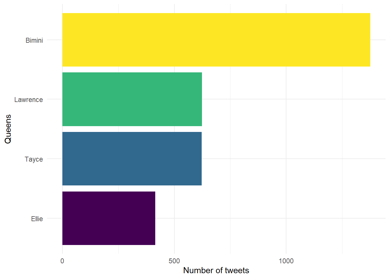
dat_token %>%
  filter(word %in% c("teamlawrence", "teambimini", "teamtayce", "teamellie"))%>%
  count(word, sort = TRUE) %>%
  head(20) %>%
  mutate(word = str_to_title(word),
         word = reorder(word, n))%>%
  ggplot(aes(x = word, y = n, fill = word)) +
  geom_col(show.legend = FALSE) +
  coord_flip()+
  scale_y_continuous(name = "Number of tweets")+
  scale_x_discrete(name = "Queens") +
  theme_minimal() +
  scale_fill_viridis_d()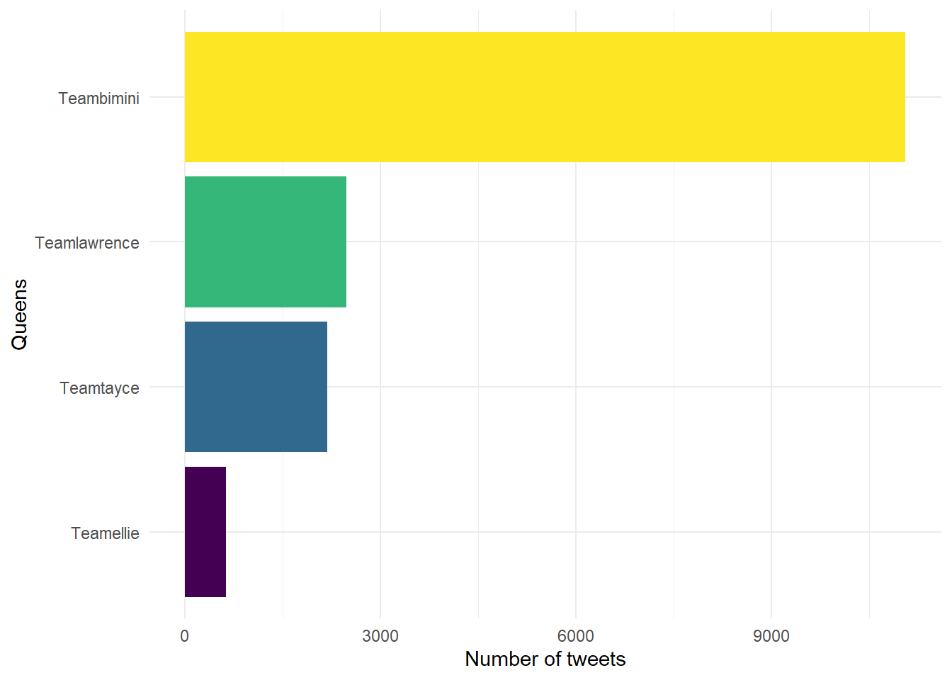
The next lot of code runs a sentiment analysis on the tweets that each Queen is mentioned in. Sentiment analyses using existing ratings of words (e.g., if they’re positive or negative) to give you a sense of whether the queen is being mentioned in a tweet that is overall positive or negative in tone. Again it’s not perfect, it can’t cope with slang (e.g., it will think that a sickening death drop is a bad thing), but it does have face validity.
# do a sentiment analysis for each queen

bimini <- dat_mentions %>%
  filter(bimini == "TRUE")%>%
  inner_join(get_sentiments("bing"))%>%
  count(index = tweet, sentiment) %>%
  spread(sentiment, n, fill = 0) %>%
  mutate(sentiment = positive - negative)%>%
  mutate(queen = "bimini")

lawrence <- dat_mentions %>%
  filter(lawrence == "TRUE")%>%
  inner_join(get_sentiments("bing"))%>%
  count(index = tweet, sentiment) %>%
  spread(sentiment, n, fill = 0) %>%
  mutate(sentiment = positive - negative)%>%
  mutate(queen = "lawrence")

tayce <- dat_mentions %>%
  filter(tayce == "TRUE")%>%
  inner_join(get_sentiments("bing"))%>%
  count(index = tweet, sentiment) %>%
  spread(sentiment, n, fill = 0) %>%
  mutate(sentiment = positive - negative)%>%
  mutate(queen = "tayce")

ellie <- dat_mentions %>%
  filter(ellie == "TRUE")%>%
  inner_join(get_sentiments("bing"))%>%
  count(index = tweet, sentiment) %>%
  spread(sentiment, n, fill = 0) %>%
  mutate(sentiment = positive - negative)%>%
  mutate(queen = "ellie")

# combine sentiment analysis for each queen into one tibble and then calculate total positive, negative
# and overall sentiment scores for each queen

dat_sentiment <- bind_rows(lawrence, ellie, bimini, tayce) %>%
  group_by(queen) %>%
  summarise(positive = sum(positive),
            negative = sum(negative),
            overall = sum(sentiment))%>%
  gather(positive:overall, key = type, value = score)%>%
  mutate(type = factor(type, levels = c("positive", "negative", "overall")))%>%
  mutate(queen = factor(queen, levels = c("lawrence", "ellie", "bimini", "tayce")))

# display table of sentiment scores

tbl <- dat_sentiment %>%
  spread(type, score)%>%
  arrange(desc(overall))

grid.table(tbl)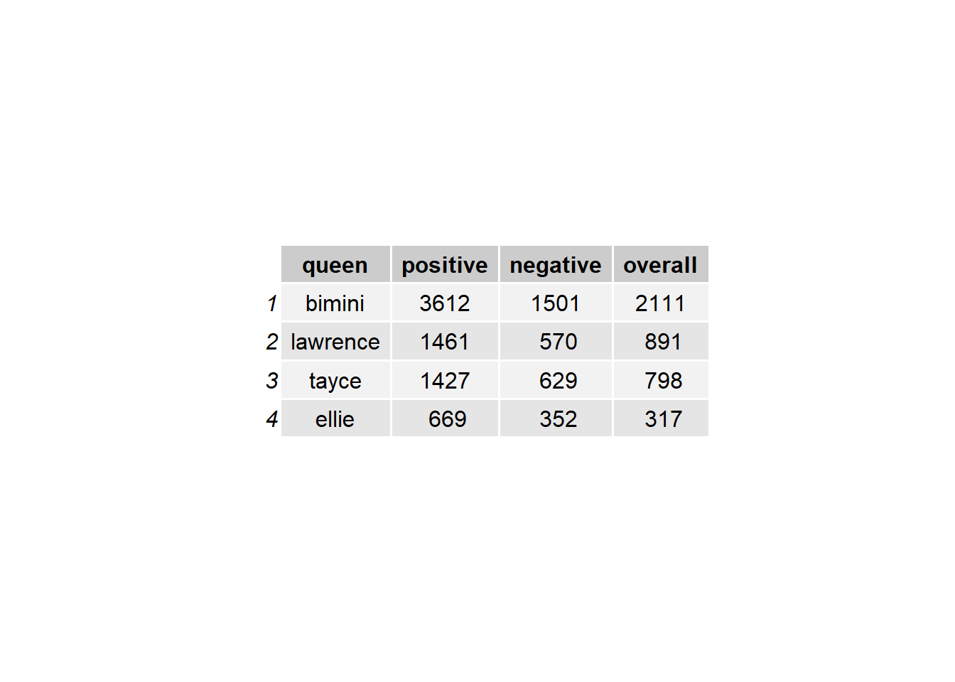
# create plot of the sentiment scores by each queen, ordered by overall score

ggplot(dat_sentiment, aes(x = type, y = score, fill = type)) +
  stat_identity(geom = "bar", position = "dodge", show.legend = FALSE)+
  facet_wrap(~ queen, ncol = 3)+
  coord_flip()+
  scale_fill_manual(values = c("positive" = "green", "negative" = "red", "overall" = "blue"))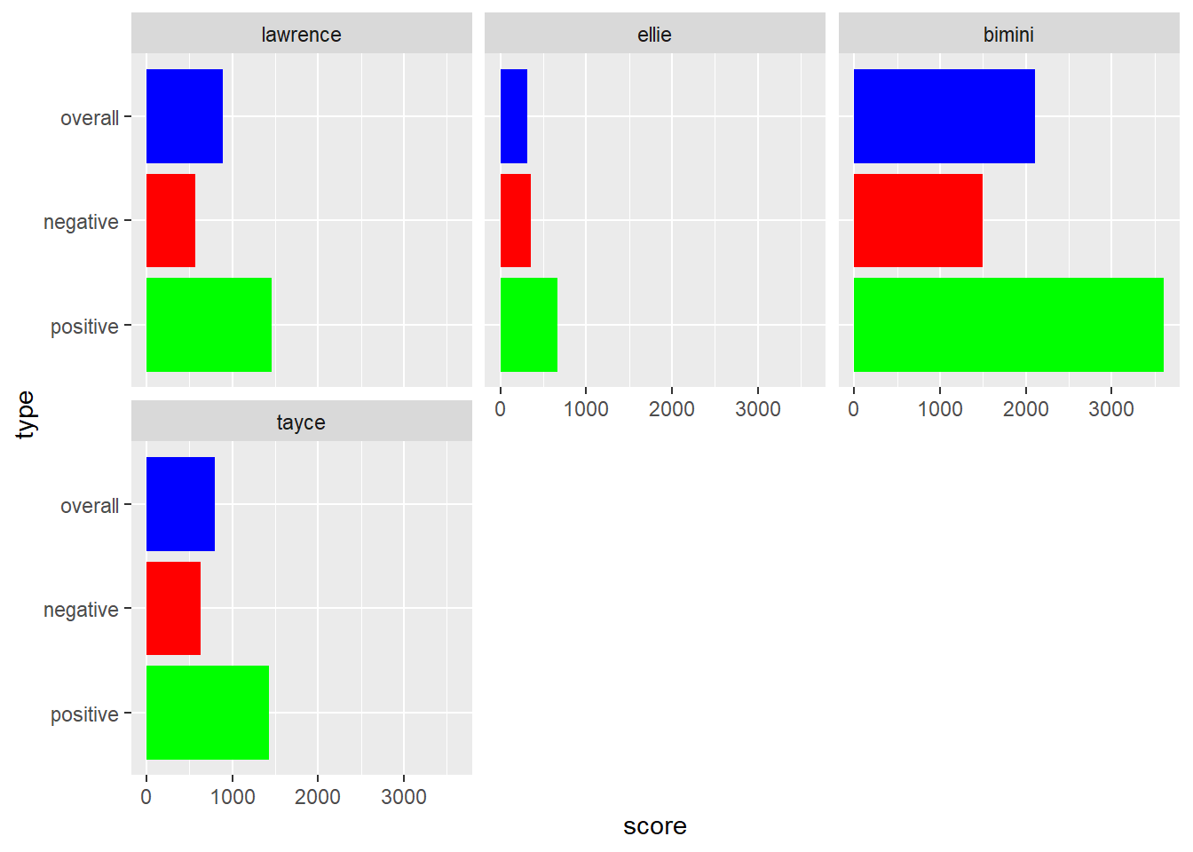
Emily Nordmann
Senior Lecturer in Psychology
I am a teaching-focused Senior lecturer and conduct research into the relationship between learning, student engagement, and technology.